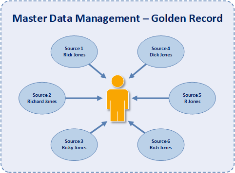
Master Data Management “The Golden Record”

The Golden Record is a fundamental concept within Master Data Management (MDM) that identifies and defines the single version of truth, where truth is understood to be data that is trusted to both accurate and correct. When building database tables from disparate data sources, there commonly are issues of duplication of records, incomplete values within a record, and records with poor data quality. The golden record solves these issues by correcting duplications, by providing values when a value may not exist, and by improving data quality within a record. Moreover, the Golden Record is a record that an organization assumes to best possible record to be utilized.

The main consideration in the creation and maintenance of the Golden Record is the matching and merging of records that were created in different data sources. A good MDM system will include functionality to automatically merge similar records as much as possible. Additionally a good MDM system will provide functionality to allow a data steward to manually determine the best possible record. The data steward should be able to use their knowledge of a particular data set to make a judgement related to the correct values in a record. And the data steward should be able to identify whether an attribute or an entire records is correct.

Source Data From Multiple Systems

When similar records from different systems have different values, one of the records has be chosen as the one that is correct. In order to determine the correct record, either the system or the data steward will need to consider the user of each each data set, the level of quality in each data set, the attribute of each data set that are the most reliable, and the rules for determining priority for each field. In the example above, each of three systems contain a record that is similar to a record contained in the other two systems. But the values in each attribute of the three similar records are not exactly the same. The Golden Record could be determined to be an entire record from one of the source systems or a combination of attributes from the records in the source systems.

The Golden Record – The Best Choice of Attributes

In this case, the Golden Record contains a combination of values for the multiple source systems. The value for the name field is taken from source system three, while all of the values of the other attributes are taken from source system one.

Data Vault Data Model for EDW

The Data Vault data model provides an evolution in the way that enterprise data warehouses (EDW) are designed, constructed, and deployed. Moreover, Data Vault provides a new and powerful way to model data within an enterprise data warehouse (EDW) that is more scalable, extensible, and auditible than conventional modeling techniques. It is an ideal modeling technique for EDW that either have a large volume of data, a large number of disparate data sources, a high degree of variety in the ingested data, or a large number of diverse information consumers. Fundamentally, the Data Vault is a hybrid data modeling technique that provides historical data representation from multiple sources designed to be resilient to environmental changes.

The Data Vault model provides a method of looking at historical data that deals with issues such as auditing, tracing of data, loading speed and resilience to change as well as emphasizing the need to trace where all the data in the database came from. This means that every row in a data vault is accompanied by record source and load date attributes, enabling an auditor to trace values back to the source.

According to Dan Linstedt, creator of Data Vault data modeling, Data Vault is defined as:

The data vault is a detail oriented, historical tracking and uniquely linked set of normalized tables that support one or more functional areas of business. it is a hybrid approach encompassing the best of breed between 3rd normal form (3nf) and star schema. the design is flexible, scalable, consistent and adaptable to the needs of the enterprise. it is a data model that is architected specifically to meet the needs of today’s enterprise data warehouses.

Data Vault Tables

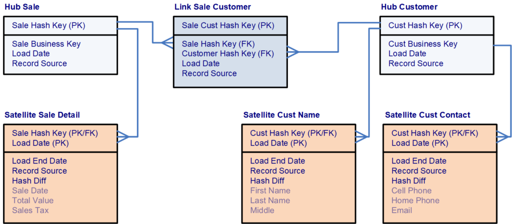
The Data Vault model is based upon three distinct table types which each table type serving a specific purpose:

•  Hub tables store a unique field for each business entity known as business key.
•  Link tables store relationships between hub tables.
•  Satellite tables store the attributes of the business key.

Hub Table:
Consists of a list of unique business keys that represent a distinct way of identifying a business element as well as fields that describe the origin of the record. Additionally hub tables cannot contain any foreign key fields. Types of fields included in the hub table are:

1) Hash Key which serves as the primary key of the hub table in a hash format.
2) Load Date which includes the date time that the record was inserted into the hub table.
3) Record Source which includes the name of the data source from where the record originated.
4) Business Key which is the unique identifier of the business entity as a either a text or number value and can be more than one field in the table.

Link Table:
Establishes relationships between business keys, contains foreign keys to hub tables, and includes fields about the relationship. A link table is therefore an intersection of business keys and contains the fields that represent the business keys from the related hub tables. The purpose of the link table is to capture and record the relationship of data elements at the lowest possible level of granularity. And a link table must have relationship with at least two hub tables. Types of fields included in link table are:

1) Hash Key which serves as the primary key of the link table in a hash format.
2) Foreign Keys which provide references to the primary hash key of related hub tables.
3) Business Keys which provide a copy of the business key value from the related hub tables.
4) Load Date which includes the date time that the record was inserted into the link table.
5) Record Source which includes the name of the data source from where the record originated.

Satellite Table:
Comprised of all the fields that describe a business entity or relationship and provide context at a given time or over a time period to either a hub or link. Satellite tables consist of foreign keys linking them to a parent hub table or link table, fields that describe the origin of the record, as well as a start and end dates fields. The structure and concept of a
satellite table is very much like a type 2 slowly changing dimension in a dimensional model. History of changes is stored within a
satellite table as well as change data capture (CDC) is conducted within a satellite table. Types of fields included in the satellite table are:

1) Parent Hash Key which provides a foreign key reference to a hub table and is one of two fields included in the primary key of the table.
2) Start Date which indicates the date and time that the satellite record starts being active and is the second of two fields included in the primary key of the table.
3) Record Source which includes the name of the data source from where the record originated.
4) Load End Date which indicates the date and time that the satellite record became inactive.
5) Extract Date which indicates the date and time that the records was extracted from the source system.
6) Hash Diff which is a hash value of all of the descriptive values of a record.
7) Descriptive Fields which are any fields that provide more detail about the entity.

Business Keys and Hash Keys

Business Key: A text value that must be a declared unique or alternate key constraint within the hub table. This means that only one distinct value can exist within the entire Hub table. The business key does not necessarily have to be just one field within the hub table. It can be a compound key made up of more than one column. Business keys are also included as non-unique fields within link tables. True business keys are not tied to any one source system and could be contained within multiple source systems. Examples of typical business keys include: account number, product code, customer number, employee id, invoice number, and order number.

Hash Key:  One of the innovations within the latest version of the Data Vault model is the replacement of standard integer primary keys or surrogate keys with hash-based primary keys. This feature of the Data Vault model enables a Data Vault solution to be deployed either on a relational data management system (RDBMS) or on Hadoop systems. Hadoop systems do not have surrogate key generators like an RDBMS, but a unique MD5 hash value can be generated in Hadoop. With a hash key being used in Hadoop and a hash key being used in an RDBMS, tables can be logically joined.

Data Vault and Information Marts

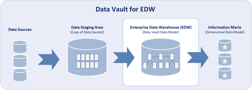
The Data Vault layer within an EDW is normally used to store data and data is never deleted from the data vault unless there is a technical error while loading data. Additionally the Data Vault layer is not optimized for business intelligence and analytical use. Dimensional modeling is much more suited for this purpose. Subsequently, information marts contain dimensional models and are the source for data analytics. In order to be used by end-users, data contained in the data vault needs to be converted to a dimensional model and moved into related information marts. Dimension tables in information marts will then be sourced from data vault hub and related satellite tables. While fact tables in information marts will be sourced from data vault link and related satellite tables. Upon data being converted into dimensional models and moved into information marts, business intelligence tools including SAP Business Objects, Cognos, OBIEE, Tableau, SSAS, Power BI, & Qlik Sense can be used by end-users to conduct analytics on the data.

Summary

The best use for the Data Vault data model is within the enterprise data warehouse (EDW) of a complete business intelligence environment. Moreover, the Data Vault model is specifically designed for this purpose. And the Data Vault model is the ideal data modeling technique for databases that store large volumes of highly volatile data, contain a high degree of data variety, and contain data from multiple disparate sources.

However, the Data Vault model is only one part of the complete Data Vault architecture which contains three layers:

1) Data Staging Area which contains a copy of source data.
2) EDW which is designed using the Data Vault model.
3) Information Marts which are designed using a dimensional model are the source of data for end-user analysis.

DevOps / DevSecOps – Rapid Application Development

About DevOps

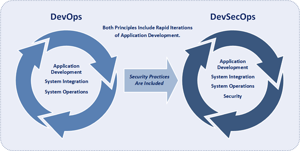
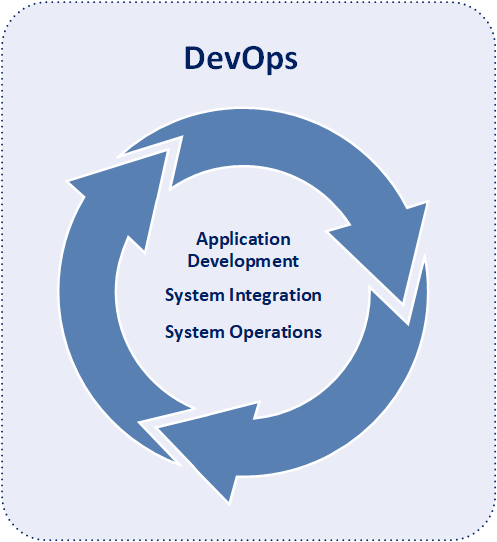
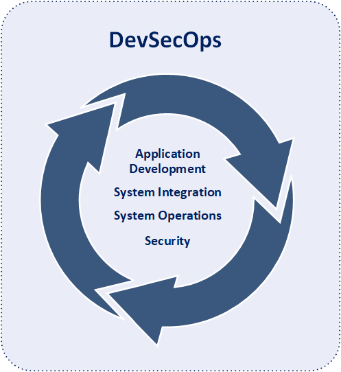
DevOps is a software development paradigm that integrates system operations into the software development process. Moreover, DevOps is the combination of application development, system integration, and system operations. With DevOps development and technical operations personnel collaborate from design through the development process all the way to production support.

Dev is short for development and includes of all the personnel involved in directly developing the software application including programmers, analysts, and testers. Ops is short for operations and includes all personnel directly involved in systems and network operations of any type including systems administrators, database administrators, network engineers, operations and maintenance staff, and release managers.

The primary goal of DevOps to enable enhanced collaboration between development and technical operations personnel. Benefits include more rapid deployment of software applications, enhanced quality of software applications, more effective knowledge transfer, and more effective operational maintenance.

A fundamental practice of DevOps is the delivery of very frequent but small releases of code. These releases are typically more incremental and rapid in nature than the occasional updates performed under traditional release practices. Frequent but small releases reduce risk in overall application deployments. DevOps helps teams address defects very quickly because teams can identify the last release that caused the error. Although the schedule and size of releases will vary, organizations using a DevOps model deploy releases to production environments much more often than organizations using traditional software development practices.

The essential concepts that make DevOps an effective software development approach are collaboration, automated builds, automated tests, automated deployments, & automated monitoring.  Moreover, the inclusion of automation into DevOps fosters speed, accuracy, consistency, reliability, and speed of release deployments.  Within DevOps, automation is utilized at every phase of the development life cycle starting from triggering of the build, carrying out unit testing, packaging, deploying on to the specified environments, carrying out build verification tests, smoke tests, acceptance test cases and finally deploying on to a production environment. Additionally within DevOps, automation is also included in operations activities, including provisioning servers, configuring servers, configuring networks, configuring firewalls, and monitoring applications within the production environments.

About DevSecOps

DevSecOps is a software development paradigm of integrating security practices into the DevOps process. SecOps is short for security operations and includes the philosophy of completely integrating security into both software development and technical operations as to enable the creation of a “Security as Code” culture throughout the entire IT organization. DevSecOps merges the contrasting goals of rapid speed of delivery and the deployment of highly secure software applications into one streamlined process. Evaluations of the security of code are conducted as software code is being developed. Moreover, security issues are dealt with as they become identified in the early parts of the software development life cycle rather than after a threat or compromise has occurred.

DevSecOps reduces the number of vulnerabilities within deployed software applications and increases the organization’s ability to correct vulnerabilities.

Before the use of DevSecOps, organizations conducted security checks of software applications at the last part of the software development life cycle. By the time performed security checks were performed, the software applications would have already passed through most of the other stages and would have been almost fully developed. So, discovering a security threat at such a late stage meant reworking large amounts of source code, a laborious and time-consuming task. Not surprisingly, patching and hot fixes became the preferred way to resolved security issues in software applications.

DevSecOps demands that security practices be a part of the product development lifecycle and be integrated into each stage of the development life cycle.  This more modern development approach enables security issues to be identified and addressed earlier and more cost effectively than is possible with a conventional and more reactive approach.  Moreover, DevSecOps engages security at the outset of the development process, empowers developers with effective tools to identify and remediate security findings, and ensures that only secure code is integrated into a product release.

Continuous Integration / Continuous Delivery (CI/CD) Processes

Continuous Integration (CI)

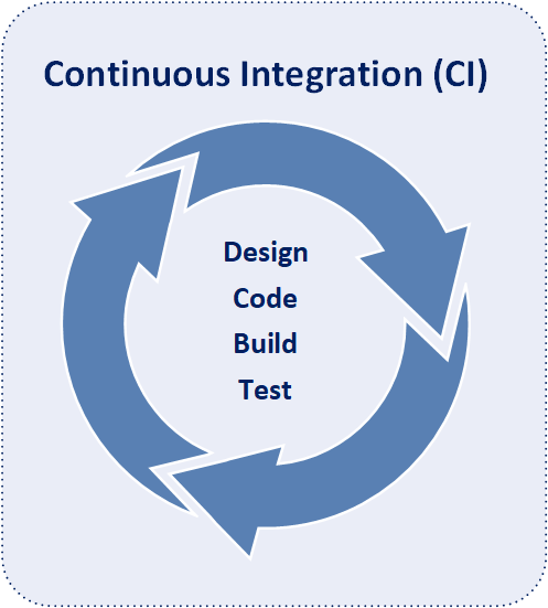
Continuous Integration is a practice utilized by software development teams in which the merging and testing code of code is automated, and code is constantly being integrated into a shared code repository. The merging of code into the shared repository occurs at short intervals and can occur several times within a day. Moreover, each small integration of code is commonly verified by an automated build and by automated tests. While automated testing is not required as part of CI, it is typically implied.

The primary goal of CI is the establishment of a consistent and automated way to build and test custom software applications. Further, CI enables development teams to effectively collaborate in the development of components of a complete software application and can improve the overall quality of the application code. And with CI in place, development teams are more likely to frequently share codes changes rather than waiting for the end of a development cycle.  Implementing CI also helps development teams catch bugs early in the development cycle, which makes them easier and less expensive to fix.  

Continuous Delivery (CD)

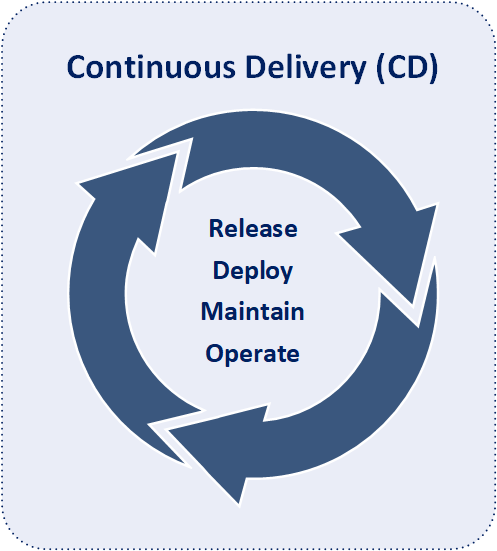
Continuous Delivery is the next step after CI in the software development process in which code changes are automatically migrated to the next infrastructure environment (i.e. Test, Acceptance, Pre-Production, Beta, Production, etc.). Application code is typically developed and integrated together within a development environment. CD then automates the delivery of software applications to another infrastructure environment after the code is successfully built and tested. CD is not limited to one environment and typically includes three to four environments. In addition to the automated migration of software applications to another environment, CD performs any necessary service calls to web servers, application servers, databases, and other services that may need to be restarted or follow other procedures when applications are migrated to that environment.  

Whereas CI focuses on the build and the unit testing part of the development cycle for each release, CD focuses on what happens with a compiled change after it is built. In CD, code automatically moves through multiple test, acceptance, and/or pre-production environments to test for errors and inconsistencies as well as to prepare the code for a release to a production environment. Within the CD process, tests are automated and software packages rapidly deployed with minimal human intervention.

Between CI and CD Processes

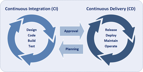
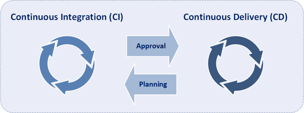
The transition between the CI and CD processes is both seamless and rapid. As the CI process ends, the CD process immediately starts. And when the CD process end, the CI process starts again. After software builds are successfully tested within the CI process, an approval kicks off the subsequent related CD process. Further, approvals can be either automatically executed with the success of all automated unit tests or manually executed with a human agreeing that all unit tests are successful. Then upon completion of the CD process, planning immediately starts for the next iteration of the CI process Typically planning focuses on the scope and tasks involved with the development of the next software component.

Complete CI/CD Process

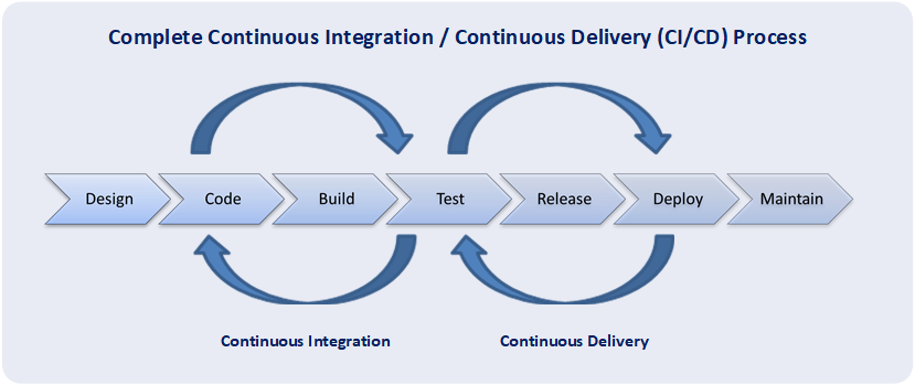
The Complete Continuous Integration / Continuous Delivery (CI/CD) Process is a way of developing software which code is constantly being both developed and deployed. Updates to software modules can occur at any time and occur in a sustainable way. CI/CD enables organizations to develop software quickly and efficiently with a seamless gap between development and operations. Moreover, CI/CD leverages a complete process for continuously delivering code into production, and ensuring an ongoing flow of new features and bug fixes. Many development teams find that the CI/CD approach leads to significantly reduced integration problems and allows a team to develop quality software in a rapid fashion. The approach is also flexible enough to let code releases occur on a schedule (i.e. weekly, bi-weekly, monthly, etc.). Both rapid release of code and scheduled release of code can occur within a complete CI/CD process.

Commonly Used Machine Learning Algorithms & Techniques

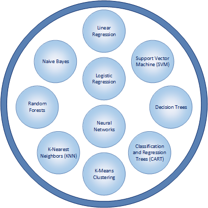
Just as there are numerous practical applications of machine learning, there are also a wide variety of algorithms and statistical modeling techniques that help enable implementations of machine learning to be effective. Some of the most commonly used algorithms and statistical modeling techniques for machine learning include:

1) Linear Regression: Enables the summary and study of relationships between two continuous, quantitative variables: Linear regression enables the modeling of the relationship between two variables by utilizing a linear equation (i.e. y = f(x)). One variable is considered to be an explanatory variable, and the other is considered to be a dependent variable. Linear regression is one of the most basic ways of conducting statistical modeling and is typically one of the first ways that is utilized.

2) Logistic Regression: Analyzes data in which there are one or more independent variables that determine an outcome. The outcome is measured with a binary or dichotomous variable (usually in the format of 0 and 1). Logistic regression focuses on estimating the probability of an event occurring based on the data that has been previously provided. And the goal of logistic regression is to find the best fitting model to describe the relationship between the dichotomous dependent variable and a set of independent variables.

3) Decision Trees: Uses observations about certain actions and identifies an optimal path for arriving at a desired outcome. Decision trees model decisions and their possible consequences in a binary tree-like format with two conditions for each decision. A decision tree is a flowchart-like structure that enable analysis to go from observations about an item to conclusions about the item’s target value. Observations are represented in the branches while conclusions are represented in leaves. The paths from tree root to individual leaves represent classification rules.

4) Classification and Regression Trees (CART): Two similar ways of conducting an implementation of decision trees. Rather than using a statistical equation, a binary tree-structure is constructed and is used to determine an outcome. Classification trees are used when the predicted outcome is the grouping of data to which the data belongs. Regression tree are used when the predicted outcome contains a numeric or real number value (e.g. the price of a car, salary amount, value of a financial investment).

5) K-Means Clustering: Used to categorize data without previously defined categories or groups. The algorithm works by finding groups with similar characteristics within the data, with the number of groups represented by the user-defined variable K. And the groups of data are known as clusters. The modeling technique then works in an iterative manner to assign each data point to one of K clusters.

6) K-Nearest Neighbors (KNN): Estimates how likely a data point is to be a member of one group or another. Predictions are made for a data point by searching through the entire data set to find the K-nearest groupings of data with related characteristics to the data point. The groupings of data with related common characteristics that are similar to the characteristics of the data point are known as neighbors. The value of K is user-specified and a similarity measure or distance function is used to determine how close neighbors are to each other.

7) Random Forests: Combine multiple algorithms to generate better results for classification and regression. Each individual classification is fairly weak. But much stronger with more accurate results when combined with other classifications. Random forests include a decision tree that incorporates random selections. Each tree is constructed using a random sample of records and each split is constructed using a random sample of variables. The number of variables to be searched at each split point is user-specified.

8) Naive Bayes: Classifies every value as independent of any other value and is based upon the Bayes theorem of calculating probability. Further, the algorithm enables a classifications or groupings of data to be predicted, based on a given set of variables and probability. A Naive Bayesian model is fairly easy to build, with no complicated iterative parameter estimation. It is particularly useful for very large data sets.

9) Support Vector Machine (SVM): A method of classification in which data values are plotted as points on a graph. The value of each feature of the data is then identified with a particular coordinate on a graph. SVM includes the construction of hyperplanes on a graph which assists in the identification of groupings of data, relationships between data, and data outliers.

10) Neural Networks: Loosely designed on the human brain and includes the sophisticated ability to recognize patterns. Neural networks utilize large amounts of data to identify correlations between many variables. Moreover, neural networks possess the ability the to learn how to process future incoming data. The patterns that neural networks recognize are numerical and contained in vectors. And vectors are the mathematical translation of all real-world data including voice, graphics, sounds, video, text, and time. Neural networks are very effective in learning by example and through experience. They are extremely useful for modelling non-linear relationships in data sets and when the relationship among the input variables is difficult to determine.

Categories of Machine Learning Algorithms

At the core of machine learning are computer algorithms, which are procedures for solving a mathematical problem in a finite number of steps. And machine learning algorithms are utilized to build a mathematical model of sample data, known as “training data”. Machine learning algorithms can be divided into categories according to their purpose. The main categories of machine learning algorithms include:

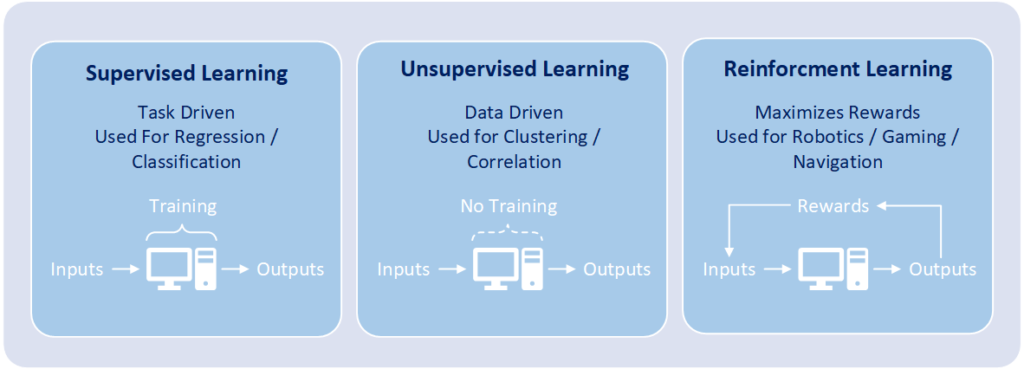
1) Supervised Learning: Each algorithm is designed and trained by human data scientists with machine learning skills, and the algorithm builds a mathematical model from a data set that contains both the inputs and the desired outputs. The data scientist is responsible for determining which variables, or features, the mathematical model should analyze and use to develop predictions. A supervised learning algorithm analyzes sample or “training data” and produces an inferred function. The process of setting up and confirming a mathematical model is known as “training”. Once training is complete, the algorithm will apply what was learned to new data. Through the use of modeling techniques including classification, regression, prediction, and gradient boosting, supervised learning uses patterns to predict the values on additional data sets. Supervised learning is commonly used in applications where historical data predicts likely future events such as language recognition, character recognition, handwriting recognition, fraud detection, spam detection, and marketing personalization. Algorithms related to classification and regression utilize this category of learning.

2) Unsupervised Learning: Without setup from a human data scientist and without reference to known or desired outcomes, each algorithm infers patterns from a data set Thus the algorithm contains inputs but no previously determined outcomes. Further the algorithm utilizes an iterative approach called deep learning to review data and arrive at conclusions. Additionally, unsupervised learning algorithms are used to find structure in the data, which includes grouping, categorization, and clustering of data. Unsupervised learning algorithms work by analyzing millions records of data and automatically identifying hard to find correlations between data within the data set. These types of algorithms have only become feasible in the age of big data, as they require massive amounts of data to be useful in making predictions. Fundamentally, unsupervised learning conducts analysis on massively sized data sets, to discover useful patterns in the data, and then group the data into unique categories. The main types of unsupervised learning algorithms include clustering algorithms and association rule learning algorithms. Unsupervised learning is often used for grouping customers by purchasing behavior and correlations between purchases (i.e. people that buy X also tend to buy Y).

3) Reinforcement Learning:Through numerous iterations, the machine is trained to make the best possible decisions. The algorithm discovers through trial and error over many attempts which actions yield the greatest rewards. Steps that produce positive outcomes are rewarded and steps that produce negative outcomes are penalized. Subsequently reinforcement learning includes the sequence of decisions and acts like a game is being played. The objective of the mathematical model is for the decision-maker to choose actions that maximize the expected reward over a given amount of time. The decision-maker will most optimally reach the goal by following a good policy. And it is up to the model to determine the policy that figures out how to perform the task to maximize the reward. The policy is determined by starting from totally random trials and finishing with sophisticated tactics. Reinforcement learning is often used for robotics, gaming, and navigation.

Definition and Examples of Machine Learning

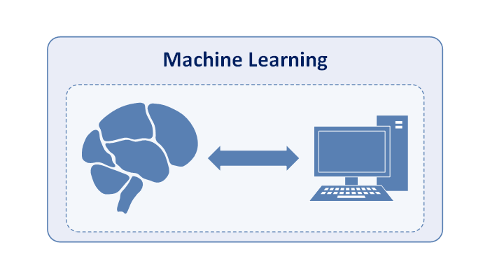
Machine Learning  is a combined application of both data analysis and artificial intelligence that provides computer systems the ability to automatically learn and improve from experience without being explicitly programmed. The fundamental idea of machine learning is that computer systems can effectively identify patterns in data and make decisions with minimal human intervention. Moreover, machine learning focuses on discovering correlation between data elements, recognizing data patterns, and performing tasks without additional human instructions. Because machine learning often uses an iterative approach to learn from data, the learning routines and processes can be easily automated. 

Fundamentally, machine learning is focused on the analysis of data for structure, even if the structure is not known ahead of time. Moreover, machine learning is focused on the implementation of computer programs and systems which can teach themselves to adapt and evolve when introduced to new data. At the core of machine learning are computer algorithms, which are procedures for solving a mathematical problem in a finite number of steps. And machine learning algorithms are utilized to build a mathematical model of sample data, known as “training data”.

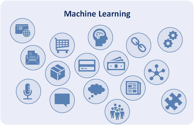
Today machine learning is being used in a wide range of applications. Some common examples of how machine learning is currently being used include:

•  Social Media News Feeds and People You May Know
•  Virtual Personal Assistants / Chatbots
•  Product Recommendations / Market Personalization
•  Credit Card Fraud Detection
•  Email Spam and Malware Filtering
•  Self-Driving Car
•  GPS Traffic Predictions
•  Audio / Voice
•  Natural Language Processing / Speech Recognition
•  Financial Trading
•  Online Search
•  Healthcare

Facebook’s News Feed is one of the best examples of machine learning that has started becoming incorporated into everyday life. When a Facebook user reads, comments on, or likes a friend’s post on his personnel feed, the news feed will re-prioritize the content on user’s feeds and show more of the friend’s post and activity at the beginning of the feed. Should the member no longer read, like, or comment on the friend’s posts, the news feed will again re-prioritize the feed and will adjust the posts that appear at the begin accordingly.

A number of company websites now offer the option to chat with customer support representative while using the website. But the customer does not necessarily communicate with a live human customer support representative anymore. In many cases the customer support representative is an automated chatbot. And these chatbots are able to extract information from the website, internal database, and external data sources to present answers to customer questions. Meanwhile, chatbots get better at answering questions over time. They tend to comprehend the user questions better and respond to customers with more relevant, accurate and useful answers.

Many organizations want to gain advantage over financial markets and accurately predict market activity and fluctuations. More and more financial trading firms are using sophisticated systems to predict and execute trades at high speeds and high volume. The systems are able to predict market activity which enables effective execution of market trades (i.e. buys and sells). Computer systems have a big advantage over humans in consuming vast quantities of data and rapidly executing a large number of trades.

Data Science – Discovering Information from Data

Data science is a broad field that refers to the collective processes, theories, concepts, tools and technologies that enable the ability to gain knowledge and insights from all forms of raw data. Further, data science combines different fields of work, techniques, and disciplines in order to interpret data for the purpose of decision making. It employs techniques and theories drawn from many fields within the context of mathematics, statistics, information science, and computer science. However, Data science is ultimately about analyzing data in creative, methodical, and sophisticated ways to generate business value.

Much like science is a generic term that includes a number of specialties and disciplines, data science is a broad term for a variety of techniques to discover information from sets of data. Included in data science are techniques of scientific method, mathematics, statistics, computer programming, machine learning, data analysis, and business analysis. If it is a technique performed on data to analyze it or discover information from data, it most likely falls within the field of data science.

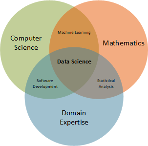
The most basic disciplines that make up the field of data science are computer science, mathematics, and domain expertise. And where the basic disciplines intersect, data science also includes cross-functional disciplines of machine learning, statistical analysis, and software development.

Each of the basic disciplines within data science are defined as:

•  Computer Science: Encompasses both the theoretical study of algorithms (i.e. well-defined procedures that allows a computer to solve a problem), and the practical problems involved in implementing algorithms in terms of digital computer hardware and software.
•  Mathematics: The study of the measurement, properties, and relationships of quantities and sets, using numbers and symbols including arithmetic, algebra, geometry, and calculus.
•  Domain Expertise: Deep understanding and knowledge in a specific business area, business process, business area, business function, or technical subjects for a project or program.

Each of the cross-functional disciplines within data science are defined as:

•  Machine Learning: An application of artificial intelligence that provides systems the ability to automatically learn and improve from experience without being explicitly programmed.
•  Statistical Analysis: Science of collecting, exploring and presenting large amounts of data in order to discover probability, relationships, correlation, and trends.
•  Software Development: Process of designing, programming, & deploying executable computer programs for the purpose of accomplishing a specific computing task.

With the use of many techniques and tools, data science can add value to any organization in any industry that would like to utilize their data to make better decisions. And the goal of data science is to construct the means for extracting business-focused insights from data. Fundamentally, data science utilizes a variety of sophisticated techniques and tools to conduct analysis on large and varied data sets for the purpose of generating useful information.

Search Engine NoSQL Database

Search Engine NoSQL Database

Search engine databases are NoSQL databases that deal with data that does not necessarily conform to the rigid structural requirements of relation database management systems (RDBMS) as data for search may be text-based, semi-structured, or unstructured. Search engine databases are made to help users quickly find information they need in a high-quality and cost-effective manner. They are optimized for key word queries and typically offer specialized methods such as full-text search, complex search expressions, and ranking of search results.

Search engine databases contain two main components. First content is added to the search engine database index. Then when a user executes a query, relevant results are rapidly returned utilizing the search engine database index. Fast search responses are possible because instead of searching the text directly, queries perform searches against an index. This is the equivalent of retrieving pages in a book related to a keyword by searching the index at the back of a book, as opposed to searching each of the words in each page of the book. This type of index is known as an inverted index, because it converts a page-centric data structure to a keyword-centric data structure.

Search engine databases commonly support the following types of search functionality:

•  Full-text search:  Compares every word of the search request against every word within a file. Examines all the words in every stored file that contains natural language text such as English, French, or Spanish. And is appropriate when data to be discovered is mostly free-form text like that of a news article, academic paper, essay, or book.
•  Semi-structured search:  Searches of data that have both the rigid structure of an RDBMS and full-text sentences like those in a MS Word or PDF document as they can be converted to either XML or JSON format. Semi-structured data is a form of data that has a self-describing structure and contains tags or other markers to separate semantic elements and enforce hierarchies of records and fields within the data.
•  Geographic search:  Associates locations to web resources in order to answer location-based queries. Search results will not only be related to the topic of a query, but they will also be related to a physical location associated with the query. Thus, physical locations will be retrieved are in proximity of the search topic.
•  Network search:  Offers a relationship-oriented approach to search that lets users explore the connections in data within stored documents. This can include linkages between people, places, preferences, & products and is useful in discovering relevance of relationships. The search engine processes natural language queries to return information from across network graphs
•  Navigational search:  Augments other search capabilities with a guided-navigation system allowing users to narrow down search results by applying multiple filters based on classification of items. Navigational search uses a hierarchy structure or taxonomy of categories to enable users to browse information by choosing from a pre-determined set of categories. This allows a user to type in a simple query, then refine their search options by either navigating or drilling down into a category.
•  Vector search:  Ranks document results based upon how close they are to search keywords utilizing multi-dimensional vector distance models. Vector search is a way to conduct “fuzzy search”, i.e. a way to find documents that are close to a keyword. They help find inexact matches to documents that are “in-the-neighborhood” of search keywords.

Wide Column / Column Family NoSQL Database

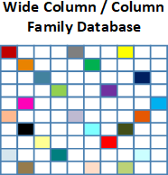
Wide Column / Column Family Database

Wide column / column family databases are NoSQL databases that store data in records with an ability to hold very large numbers of dynamic columns. Columns can contain null values and data with different data types. In addition, data is stored in cells grouped in columns of data rather than as rows of data. Columns are logically grouped into column families. Column families can contain a virtually unlimited number of columns that can be created at run-time or while defining the schema. And column families are groups of similar data that is usually accessed together. Additionally, column families can be grouped together as super column families.

The basis of the architecture of wide column / column family databases is that data is stored in columns instead of rows as in a conventional relational database management system (RDBMS). And the names and format of the columns can vary from row to row in the same table. Subsequently, a wide column database can be interpreted as a two-dimensional key-value.  Wide column databases do often support the notion of column families that are stored separately. However, each such column family typically contains multiple columns that are used together, like traditional RDBMS tables. Within a given column family, all data is stored in a row-by-row fashion, such that the columns for a given row are stored together, rather than each column being stored separately.

Since wide column / column family databases do not utilize table joins that are common in traditional RDMS, they tend to scale and perform well even with massive amounts of included data.  And databases with billions of rows and hundreds or thousands of columns are common.  For example, a geographic information systems (GIS) like Google Earth may a row ID for every longitude position on the planet and a column for every latitude position.  Thus, if one database contains data on every square mile on Earth, there could be thousand of rows and thousands of columns in the database. And most of the columns in the database will have no value, meaning that the database is both large and sparsely populated.