Complete Data Warehouse Appliance Solutions
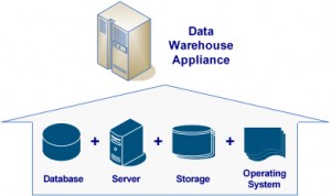
Basic Architecture of a Data Warehouse (DW) Appliance
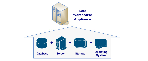
Complete data warehouse appliances are purpose-built data warehouse solutions and systems that encompass a whole-technology stack including:
• Operating System (OS)
• Database Management System (DBMS)
• Server Hardware
• Storage Capabilities

Initially DW appliances were created with proprietary custom-built hardware and storage units. Netezza, Teradata, DATAllegro, & White Cross (now Kognito) were the first vendors to provide solutions in this manner. Subsequently data warehouse appliances evolved and started to utilize lower-cost, industry-standard non-proprietary hardware components.The movement from proprietary to commodity hardware has proven to bring down the cost of the data warehouse appliance as the commodity hardware can integrated at a lower cost of both developing and integrating proprietary hardware. Examples of commodity hardware typically include general-purpose servers from Dell, Hewlett Packard (HP), or IBM utilizing Intel processors and popular network and storage hardware from either Cisco, EMC, or Sun.
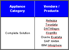
Data Warehouse Appliance - Complete Solution VendorsIntroduced 2002, Netezza was the first vendor to offer a complete data warehouse appliance, so early definitions of appliance were based upon Netezza products.  Subsequently, Netezza Performance Server still provides all of the software components of a data warehouse appliance, including the database, operating system, servers, and storage units.  However in 2009, Netezza replaced its own proprietary hardware with IBM blade servers and storage units. Further in 2010, IBM completed a corporate acquisition of Netezza.

Similar to Netezza, DATAllegro was launched in 2005 with a complete solution involving proprietary hardware. Soon after DATAllegro replaced its own proprietary hardware with commodity server from Dell and storage units from EMC. In 3008, Microsoft acquired DATAllegro in 2008 and announced it will integrate DATAllegro’s massive parallel processing (MPP) architecture into its own MS SQL Server platform, which also runs on commonly-available hardware.

Additionally, both Kognitio and Teradata replaced their proprietary hardware within their appliances in a process similar to that of DATAllegro. Kognitio now offers a row-based, in-memory database database called WX2 that does not include indexes or data partitions and runs on blade servers from IBM and Hewlett-Packard. Teradata provides a proprietary database, a variety of common operating systems (Linux, Unix, and Windows), and a proprietary networking subsystem packaged along with commodity processors and storage units.

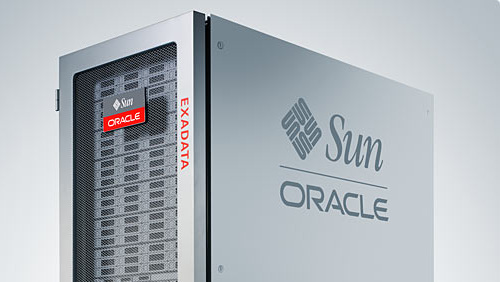
Announced at the 2008 Oracle OpenWorld conference in San Francisco, the Oracle Exadata Database Machine is a complete package of database software, operating system, servers, and storage. The product was initially assembled in collaboration between Oracle Corporation and Hewlett Packard where Oracle developed the database, operating system and storage software, while HP constructed the hardware. However, with Oracle’s acquisition of Sun Microsystems, Oracle announced the release of Exadata Version two with improved performance and usage of Sun Microsystems storage and operating systems technologies.

At the Sapphire conference in May, 2010 in Orlando, SAP announced the release of its new data warehouse appliance called HANA or High-Performance Analytic Appliance. SAP HANA is a combination of hardware, storage, operating system, management software, and in-memory data query engine that is characterized by data being held in RAM rather than being read from disks or flash storage.

Finally IBM bundles and integrates its own Infosphere Warehouse database software (formerly “DB2 Warehouse”) with its own servers and storage to deliver the IBM Infosphere Balanced Warehouse.

Share

Data Warehouse Appliance: Oracle Exadata

Announced by CEO Larry Ellison at the 2008 Oracle OpenWorld conference in San Francisco, Oracle Exadata Database Machine is a complete database appliance with support for both transactional (OLTP) and analytical (OLAP) database systems. Delivered as a complete package of database software, operating system, servers, and storage, the Oracle Exadata Database Machine is simple and fast to implement and ready for large-scale business applications.

The product was initially assembled in collaboration between Oracle Corporation and Hewlett Packard (HP) where Oracle developed the database, operating system and storage software, while HP constructed the hardware.  However, with Oracle’s acquisition of Sun Microsystems, Oracle announced the release of Exadata Version two with improved performance and usage of Sun Microsystems storage and operating systems technologies. The main idea of Exadata is to make the storage database aware and push processing of queries down to the disks for optimal scanning and performance. Subsequently an Exadata machine can scan 1 TB of data in about 3.5 seconds by scanning several (or all) disks in parallel with Oracle’s Parallel Query technology.

Oracle Exadata Database Machine

Oracle Exadata Database Machine

Currently the Oracle Exadata Database Machine provides a solution for all types of database systems, ranging from scan-intensive data warehouse applications to highly concurrent transactional applications.  With its bundled combination of storage, database software, operating system, and standard hardware components from Sun, the Oracle Exadata Database Machine provides extreme performance within a highly-available, highly-secure environment. Additionally Oracle’s unique clustering and workload management capabilities position the Oracle Exadata Database Machine to be well-suited for consolidating multiple databases onto a single and centralized environment.

Facts and Benefits of Oracle Exadata Database Machine

•  Accelerates data warehouse query performance by at least a factor of 10x.
•  Runs more queries concurrently for faster access to business-critical information.
•  Scales to 10x more concurrent users.
•  Provides a trusted highly-available and cost-effective platform.
•  Replaces and consolidates isolated special-purpose databases into one platform.
•  Allows for massive parallel processing of data with a high-bandwidth.
•  Easily expands with the connection of multiple units.
•  Includes combination of Oracle Exadata Storage server, Oracle database software, Sun Solaris operating system (OS), and the latest industry standard hardware components from Sun.
Share

Data Warehouse Appliance: SAP HANA

At the Sapphire conference in May, 2010, SAP announced the release of its new data warehouse appliance called HANA or High-Performance Analytic Appliance. SAP HANA is a combination of hardware, storage, operating system, management software, and in-memory data query engine that is characterized by data being held in RAM rather than being read from disks or flash storage. Additionally, HANA has been built to split up queries to run in parallel on multiple processors—a fundamentally different architecture from SAP’s existing applications.  This in-memory and parallel processing architecture of HANA allows for extremely fast performance of queries and analytics on very large amounts of data.

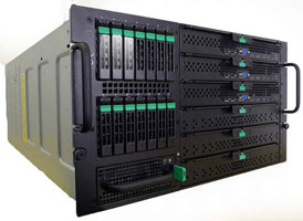
HANA Blade ServerThe SAP HANA solution has been introduced on Hewlett Packard x86 servers (HP ProLiant DL580 G7 and DL980 G7 servers) and is built upon Intel’s multi-core servers. Moreover, a single server blade can contain up to 2TB of main memory (4TB coming soon) and up to 64 processor cores.  With this total solution, SAP claims that they beat the current performance benchmark by factor of 20, on hardware that was several dozens of times cheaper for a 200X price performance improvement. SAP also claims that HANA either reduces or out-right eliminates the need for the development and deployments of complex and expensive datamarts.

SAP intends HANA systems to be well-integrated with its own enterprise resource planning (ERP) systems, allowing for transactional data in SAP ERP systems to be analyzed in real time.  However, HANA is not dependent solely on SAP ERP systems as a data source.  Moreover,  HANA is data source “agnostic”  which means most common data sources and database can be integrated with it.

According to an SAP document, the HANA platform includes a modeling environment that is simple enough for business users to work with.  Additional, HANA supports client interfaces currently include Microsoft Excel and SAP’s Business Objects business intelligence software.

References: SAP’s Transformation: A Work-In-Progress – Part One (ChainLink Research)SAP Launches HANA for In-memory Analytics (PC World)

Share

Basic Architecture of a Data Warehouse Appliance

By definition, a data warehouse appliance is a complete hardware and software solution that contains a fully integrated stack of processors, memory, storage, operating system, and database management software. The data warehouse appliance is typically constructed to be optimized for enterprise data warehouses, designed to handle massive amounts of data and queries, and designed to scale and grow over time. At its core, a data warehouse appliance simplifies the deployment, scaling, and management of the database and storage infrastructure as it provides a self-managing, self-tuning, plug-and-play database management system that can be scaled out in a modular manner.

Basic Architecture of a Data Warehouse (DW) Appliance

Basic Architecture of a Data Warehouse (DW) Appliance

Fundamentally, a data warehouse appliance is a fully-integrated solution that contains …
– Database Management System (DMBS)
– Server Hardware
– Storage Capabilities
– Operating System (OS)

The primary factor for the platform scalability and large-query optimization of the data warehouse appliance is its massively parallel processing (MPP) architecture. These MPP architectures are comprised of numerous independent processors or servers that all execute in parallel. Also known as a “shared nothing architecture”, the MPP appliance architecture is characterized by a concept in which every embedded server is self-sufficient and controls its own memory and disk operations. Further, the MPP architecture effectively distributes data amongst a number of dedicated disk storage units connected to each server in the appliance. Computations are moved as close to the data as possible and data is logically distributed amongst numerous system nodes.

Almost all large operations in the data warehouse appliance environment, including data loads, query processes, backups, restorations, and indexing are executed completely in parallel. This divide-and-conquer approach allows for extreme high performance and allows for systems to scale linearly as new processors can easily be added into the environment.

Share

Slowly Changing Dimensions – Type Four Models

Type Four – Insert Into a History Table

Type four models, also known as leveraging “history tables”, is the most technically sophisticated of the four models and may be the most difficult to implement. This modeling technique provides for nearly unlimited tracking of historical records while having less storage requirement than type two models. Rather than storing the changes in the same table, a second “history” table is created which stores only the previous values of slowly changing dimensions.

Similar to type two models, type four models accommodate infinite changes to dimensional fields and create an additional record for every change to a dimensional attribute. But in contrast to type two, type four models allow for every change to an attribute to be generated within a new record in a relatively compact history table.  The history table is subsequently more efficient in capturing a large amount of historical data.

Another key advantage of type four models is an efficient manner to query against a timeframe as the related search index only requires two fields (key and date fields).  Other modeling techniques require more fields in the search index for date queries.  Thus the search index utilizing a type four model is smaller, more intuitive, and quicker to retrieve the relevant record in the dimension table than the search index using other modeling techniques.

Type four models do have some important disadvantages.  Namely type four models require implementation of multiple tables, are less intuitive for query developers, require more effort to develop and maintain than other types of models, and allow for history tables to grow to massive size.

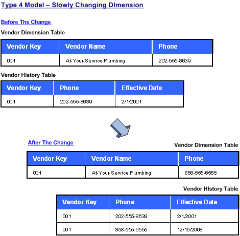
Suppose that a vendor changes his phone number to 858-555-6555 from 202-555-8639 because the phone company has added a new area code. Utilizing a type four model, the vendor dimension table would be updated and a new record will be inserted into the vendor history table in the following manner…

Type Four Model - Slowly Changing Dimension

• The vendor dimension table is updated:
– The phone number is updated from 202-555-8638 to 858-555-6555.
• A new record is inserted into the vendor history table:
– The vendor key is copied from the vendor dimension table.
– The phone number 858-555-6555 is inserted.
– The effective date of 12/15/2008 is inserted.
Share

Slowly Changing Dimensions – Type Three Models

Type Three – Leverage Previous and Current Value Fields

Type three models are defined by adding one or more columns to the dimension table, so that the new (or current or active) and old (or historical or inactive) value of an field are stored.  In addition, multiple previous values can be stored within the table depending on how many previous columns are included in the the dimension table.

Type three modeling is a middle state between complete history loss of type one models and the numerous additional records of type two models.  Moreover, type three  models only provide only a limited view of history as only a predefined number previous value of any attribute can be retained, rather than a complete history. This modeling technique is fairly useful when changes to the dimension table are made on a regular schedule, such as annually, and when archival copies of the database are stored offline for historical and audit purposes. Type three modeling is not so useful when changes are more frequent and unpredictable. Multiple previous value fields could be added to the record to provide a longer historical trail, but it may be a challenge to design the table with the optimum number of previous fields. For the most part, type three modeling makes most sense to be implemented only when only there are a limited number of previous values that need to be retained.

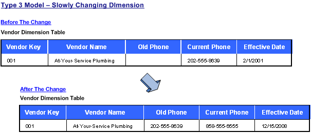
Suppose that a vendor changes his phone number to 858-555-6555 from 202-555-8639 because the phone company has added a new area code. Utilizing a type three model, the vendor dimension table will contain both a current phone and previous phone field.  Initially the vendor record contains a null value for the previous phone number and a value of 202-555-6555 for the current phone number.

Type Three - Slowly Changing Dimension

In order to process this update using the previous and current fields, the vendor dimension table is updated:
–  The previous phone field is updated to 202-555-6555, which is now the vendor’s last previous phone number.
–  The current phone field is updated to 858-555-8639, which is now the vendor’s current number.
–  The effective date is updated to the date of the change.
Share

Slowly Changing Dimensions – Type Two Models

Type Two – Update Record to Inactive / Create an Active Record

Type two modeling is a very reliable and straightforward technique for preserving history of changes to dimensional tables.  It is commonly utilized when a full or partial set of the previous values of a dimension’s attributes must be retained. In type two modeling, every time an update occurs to any of the values in a dimensional table, a new record is physically inserted as active or current into the same table and the old records are marked inactive or historical.

The main advantage of this modeling technique is that it can accommodate and record a massive amount of history and nearly an unlimited changes to slowly changing dimensions. But this advantage also can become a significant drawback. Within this modeling technique, it is possible for dimension tables to grow to massive sizes and adversely affect both system and query performance. In addition, since upon every change this modeling technique requires an update to the linked fact table, implementation is fairly difficult and may require substantial effort to design, develop, and support.

Two unique sub-methods have been established for distinguishing the active (or current) record from the inactive (or historical) records: active flagging and tuple versioning.

In the type two – active flagging sub-method, an “Active” column is constructed within the dimensional table and acts as a flag. Flags are binary fields with permissible values being Y and N, T and F, or 1 and 0. A positive value (Y, T, 1) indicates an active record, while a negative value (N, F, 0) indicates an inactive record.

Example of Type Two – Active Flagging Sub-Method

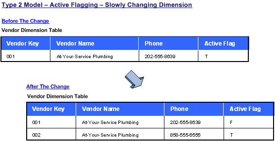
Suppose that a vendor changes his phone number to 858-555-6555 from 202-555-8639 because the phone company has added a new area code. Using active flagging, the change to the vendor dimension table would be processed as follows…

Type Two - Active Flagging - Slowly Changing Dimension

•  The current active record in the vendor dimension table is updated:
–  The active flag is changed from T to F.
–  The phone number field remains as 202-555-6555.
•  A new record is inserted into the vendor dimension table:
–  The vendor key is given the next available integer number.
–  The vendor name field remains the same as in the old record.
–  The phone number has the new value of 858-555-8639.
–  The active flag is set to T.

In the type two – tuple versioning sub-method, start date and end date columns are included on the dimension table. The values of these date fields then define the period during which that record has been active. For the most part, the start date is the date the record has been created. Moreover, the end date is the date the record has become inactive, either because a newer record has replaced it or because the original record in the source system no longer exists. On the active record, the end date will either be left null, blank, or identified in another way such as all-nines, according to modeler’s preferences and standards.

The main advantage of the tuple versioning method over active flagging is that it provides an audit trail of the date and sequence of all updates.

Example of Type Two – Tuple Versioning Sub-Method

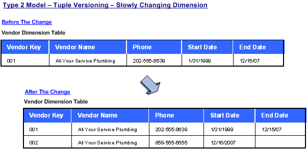
Continuing with the same example above but using the tuple versioning method, the updated phone number in a record in the vendor dimension table is processed as follows:

Type Two - Tuple Versioning - Slowly Changing Dimension

•  The current active record in the vendor dimension table is updated:
–  The end date is updated to the date of the change.
–  The phone number field remains as 202-555-6555.
•  A new record is inserted into the vendor dimension table:
–  The vendor key is given the next available integer number.
–  The vendor name field remains the same as in the old record.
–  The phone number has the new value of 858-555-8639.
–  The start date is the date the record is inserted into the table.
–  The end date is intentionally left blank.
Share

Slowly Changing Dimensions – Type One Models

Type One – Overwrite the Record

Type one modeling of slowly changing dimensions is very simple and effectively handles updates to incorrect and/or outdated values within the dimension table. Type one models do not retain a history of changes and do not store previous values in any way. With this modeling technique, the data field that has changed is simply updated to reflect the most current value.  Since this technique does not preserve any previous value, it should only be used when there is no requirement to retain historical data.

Type one models makes sense when correcting data issues, but not when the system requires retrieval of historical values. Without a doubt, type one is the simplest method for handling slowly changing dimensions. However, best practice is to utilize this technique on a very limited basis. Moreover, it should only be implemented when there is no need to track the history of changes.

Example of Type One

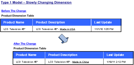
First an electronics company loads its list of products within its data warehouse. Later the company discovers that a television which was originally manufactured in the USA is now manufactured in China, and the company has in fact never received a shipment of the older American-made televisions. The product description column in the table is simply updated, and the date and time of the update is entered in the “Last Update” column.

Type One - Slowly Changing Dimension

To correct the product description, the existing description is simply overwritten with the correct value, and the “Last Update” field is revised with the current date. Moreover, the product description is updated because the item is no longer manufactured in the United States. Utilizing the type one method of managing slowly changing dimensions, the record on the product dimension table is updated in-place in the following manner…
–  The product description is updated in-place to the new description.
–  The last update is updated to the date and time of the change.
Share

What are Slowly Changing Dimensions?

Modern data warehouse design assumes that business transactions such as sales, orders, shipments, fulfillments, and receivables can occur at a rapid rate and each the details of each transaction needs to be recorded.  Hence a fact table with a dimensional model contains a separate record for each business transaction.  While in contrast, the describing or text-based values of the transaction or dimension often remain fairly constant.  Often, dimensional tables within the dimensional model do not take changes into account.

But in reality, dimensional values can and do change over time and numerous fields of a given row within a dimension table will need to be updated. This phenomenon in data modeling is known as “slowly changing dimensions” and it can be applied to any dimension table within a data warehouse schema.  Moreover, both simple and advanced modeling techniques have been established and can be implemented for handling updates and changes within a dimension table.  In addition, slowly changing dimensions assist the data warehouse in precisely recording the past values, providing an efficient method for tracking history, and allowing for the ability to respond to changes to descriptive values of transactions.

Examples of slowly changing dimensions include:
–  account name
–  customer phone number
–  vendor address
–  product description

These are good examples as they are text-based values that remain relatively constant, but can change and commonly do change over time.  Names, phone numbers, addresses are fairly intuitive and it is easy to see how these values can change slowly over time.  But let’s see how a product description could change…  A simple ingredient change or a packaging change in a product may be so trivial that the organization does not decide to give the product a new product id.  Rather the source system provides the data warehouse with a revised description of the product.  Hence the data warehouse needs to track both the old and new descriptions of the product.

Other good examples of common slowly changing dimensions are the region and territory names for a sales force. Many organizations have management that rename their region and territories on a regular basis or the management realigns their regions and territories along customer purchase patterns.   Typically the requirement of a data warehouse is to keep a record of the names of the regions and territories and the dates they were active.

Originally pioneered by Ralph Kimball, PhD, four main data modeling techniques have been established for managing dimension tables that contain slowly changing dimensions:

Type One – Overwrite the Record
Type Two – Update Record to Inactive / Create an Active Record
Type Three – Leverage Previous and Current Value Fields
Type Four – Insert Into a History Table

These four data modeling techniques range from the complete loss of historical data to an elegant but technically complex method of saving almost all historical data.  Choice of the appropriate technique by the database designer can ensure that the data warehouse contains required historical values and allows for comparisons of current data or data from other time periods.

Share

Dimensional Modeling and Data Warehouses

Dimensional modeling is a specific discipline for modeling data that is an alternative to entity-relationship (E/R) modeling. A dimension model contains the same information as an E/R model but packages the data in symmetric format whose design goals are user understandability, query performance, and resilience to change.
Ralph Kimball, PhD, The Data Warehousing Lifecycle Toolkit, 1998

Basic Dimensional Model (Star Schema)

Basic Dimensional Model (Star Schema)

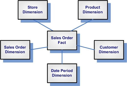
Dimensional modeling is a data modeling technique used to support on-line analytical processing (OLAP) systems and is implemented in databases that host either an enterprise data warehouses or data marts. The key point on the design of dimensional models is to resolve questions in the format “measures by dimensions.”  In addition, dimensional models are commonly referred to as star schema as they comprised of a central fact table surrounded by several dimension tables.

Within a dimensional model or star schema, there exists two types of data entities or tables
•  Facts (Measurements – Numerical Values)
•  Dimensions (Contexts and Attributes – Text, Strings, Dates, & Flags)
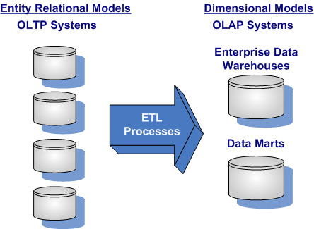
Transactional (OLTP) Systems to Analytical (OLAP) Systems

Transactional (OLTP) Systems to Analytical (OLAP) Systems

Within an enterprise data warehouse or data marts, data is fundamentally static, non-volatile and does not get updated.  Rather data is inserted or loaded in bulk into the tables in the model utilizing using batch programs or extraction, transformation, & loading (ETL) routines.  End-users of dimensional models develop queries that either read or select data, and there is no end-user inserting, updating, or deleting of data.  Data in dimensional databases requires data to be converted or extracted from on-line transactional processing (OLTP) or other OLAP systems.

The key benefits of dimensional models and data warehouses include ….
•  Separate environment from transactional systems
•  Allows for high-performance of select/read queries
•  Insulated from changes in source systems
•  Intuitive to developers and business users of queries
•  Contains data from multiple source systems
•  Optimized format for data warehouses and data marts
Share